Paper
Kauffman, S. (2022, April 22). The Variables of SU (3) x SU (2) x U (1) are Formally Capable of Collective Autocatalysis. https://doi.org/10.31219/osf.io/mdh4p
The Particle Apothecary Model (PAM)
Create your own bespoke universe. This is the current Particle Apothecary Model, PAM. Using the Gillespie algorithm, PAM studies the branching stochastic dynamical autocatalytic processes among a subset of the variables chosen from the Standard Model of Particle Physics, SU(3) x SU(2) x U(1), as these transform into one another, come into existence and vanish. PAM idealizes these variables as classical variables. This may be badly misleading. This issue needs to be assessed.
The set of transformations studied is given in Table 2, see below. In order to preserve symmetry between matter and antimatter, transformations of the pairs 7 and 8 are identical, 9 and 10 are identical, 11 and 12 are identical and 13 and 14 are identical. The “sliders” tune the rates of the different transformations. A fixed set of slider positions, each ranging between 0% - 100%, constitute that chosen set of the parameter values of the PAM model. Changing the forward and reverse transformation rates corresponds indirectly to tuning the values of the constants of the Standard Model.
The RM slider sets the background rates of a set of processes needed including the rate of entry from the vacuum of up quark – up antiquark pairs, and of down quark – down antiquark pairs. The ratio between the entry of up pairs and the entry of down pairs is set by the “energy” slider.
The HBoxT slider sets a fixed duration that is a multiple of a fixed interval approximation to the Heisenberg uncertainty relation itself proportional to dE x dT. Energy borrowed from the vacuum by the emergence from the vacuum of a quark antiquark pair is returned to the vacuum within the HBoxT interval, achieved by the vanishing of the relevant variable.
The Lifetime Extension slider sets the increased duration, hence “the delay”, in the return of the energy borrowed from the vacuum by a variable when it is “measured”.
“Delay” is the central working hypothesis that allows the autocatalytic behaviors of the variables to break matter antimatter symmetry. Later “measurement” of variables constructs spacetime, and this constitutes the new theory of Inflation here proposed.
The Mean Creation Rate slider sets the mean rate of the Poisson process by which quark antiquark pairs borrow energy and emerge from the vacuum.
The further hypothesis, beyond the fundamental PAM model, that the rate of entry of up and down quarks and antiquarks from the vacuum could depend proportionally upon the current number of these particles already in the system can be explored using the “Proportional” slider.
A random seed for each “run” of the model can be chosen and kept, or can be changed at random.
Time advances in “ticks”. At each “tick” all pending transformations are completed.
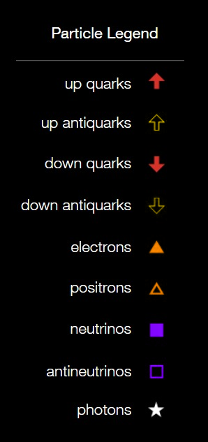
To execute a “run”, choose the PAM parameter values, choose a random seed, click “setup”, then click “go”. The resulting creation and vanishing of up and down quarks, up and down antiquarks, electrons, positrons, neutrinos, and antineutrinos are shown in the corresponding graph displays. The temporal construction of spacetime is shown on a separate display as well as a display showing a log - log and a semilog plot of spacetime construction. The goodness of fit to a power law or to an exponential temporal construction of spacetime is available by pausing or stopping a run by clicking on “go”, then clicking on “fit”. Particle density at each time moment is shown on a separate display. A panel on the right side displays the various particles present in the system at each moment. Time runs from bottom to top in this display.
The user can pause or stop a run by clicking “go” and restart the same run from the current moment by a second click on “go”. The temporal behavior at each step can be seen by clicking on “step”.
TABLE 2: TRANSFORMATIONS AMONG THE SUBSET OF THE SU(3) x SU(2) x U(1) VARIABLES FROM FIGURES 2 + 3
In each transformation the variables on the left vanish and the variables on the right appear.
1) 2 photons ->1 positron + 1 electron
2) 1 positron + 1 electron ->2 photons
3) 2 low energy photons ->1 down quark + 1 down antiquark
4) 2 high energy photons ->1 up quark + 1 up antiquark
5) 1 down quark + 1 down antiquark ->2 photons
6) 1 up quark + 1 up antiquark ->2 photons
7) 1 electron + 1 antineutrino + 1 down quark ->1 up quark
8) 1 electron + 1 antineutrino + 1 down antiquark ->1 up antiquark
9) 1 up quark ->1 down quark + 1 electron + 1 antineutrino
10) 1 up antiquark ->1 down antiquark + 1 electron + 1 antineutrino
11) 1 positron + 1 neutrino + 1 down quark ->1 up quark
12) 1 positron + 1 neutrino + 1 down antiquark ->1 up antiquark
13) 1 up quark ->1 down quark + 1 positron + 1 neutrino
14) 1 up antiquark ->down antiquark + 1 positron+ 1 neutrino
15) 2 photons ->1 muon + 1 antimuon
16) 1 muon + 1 antimuon ->2 photons
17) 1 muon + 1 antimuon ->1 electron + 1 positron
18) 1 electron +1 positron ->1 muon + 1 antimuon
19) 1 muon + 1 antimuon + 1 down quark ->1 up quark
20) 1 muon + 1 antimuon + 1 down antiquark ->1 up antiquark
21) 1 up quark ->1 down quark + 1 muon + 1 antimuon
22) 1 up antiquark ->1 down antiquark + 1 muon + 1 antimuon
23) 1 muon ->1 electron + 1 antineutrino + 1 muon neutrino
24) 1 electron + 1 antineutrino + 1 muon neutrino ->1 muon
25) 1 antimuon ->1 positron + 1 neutrino + 1 antimuon neutrino
26) 1 positron + 1 neutrino + 1 antimuon neutrino ->antimuon
